High-dimensional Spaces
In the last post we have seen examples for how numbers can encode information, becoming data. In this post we will talk about a very important way to look at data. This view will allow us to play around with data in a powerful way, and this view lies at the core of machine intelligence and the science of data.
Data samples as points in space
I have previously told you that any image can be represented by a table of numbers where each number encodes the gray scale value of the image. For the trick that I would like to teach you, this image is actually a bit too large. So for the sake of the argument, let us shrink the original 27x35 pixel image drastically until it gets really really tiny, namely 3x1, that means only 3 pixels wide and 1 pixel high - bear with me for a second even if this sounds silly to you. We won’t see anything on this image but that doesn’t matter right now. Our 3x1 image expressed in gray scale values now looks like this:
| 0.909 | 1.000 | 0.860 |
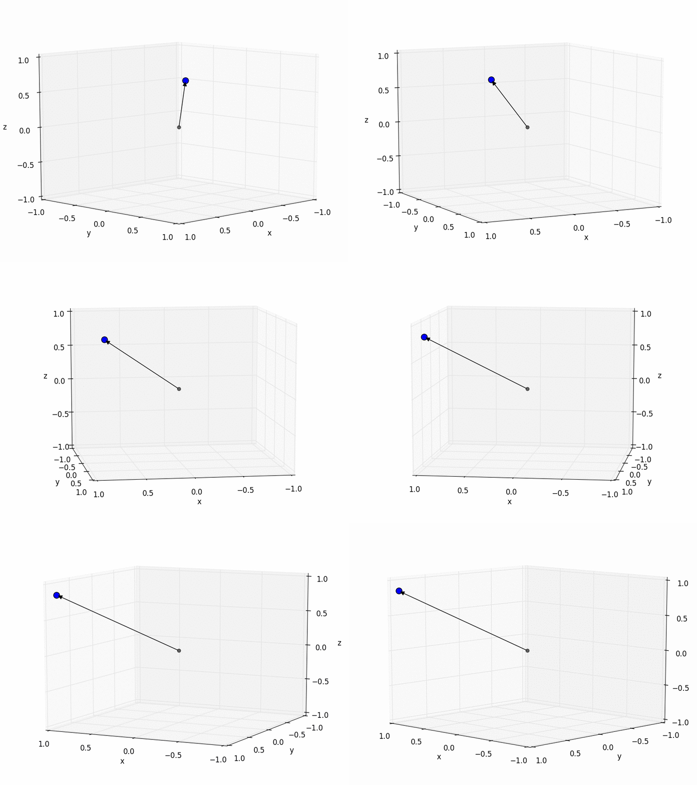
I have set the background color of each table cell to correspond to the actual gray scale value the number encodes. Here comes the trick: although we know that these three numbers encode gray scale values we can pretend they were encoding the location of a point in 3D space. So instead of encoding “luminosity” we think of the numbers are being in “meters” or “centimeters”. As you might remember from high school we draw a location as an arrow in an coordinate system. So let’s draw our 3x1 “image” in a 3D coordinate system:

So you might think: “drawing arrows is really fun but why the heck are we doing this?” There are two reasons for that: the first reason is this that we humans are really good at manipulating objects in 3D space. We know how to move objects, we know how to rotate them, how to distort and mirror them, how to project them on a 2D planar surface (by taking a picture of it), and much more. Thus, if we treat data as locations in space we can apply all our spatial 3D knowledge to it. In fact, linear algebra has got all the math worked out to simulate these 3D operations on computers (as you can admire in Toy Story, Madagascar, and so on) [1].
Now the question is, what does the 3D arrow sketched above have to do with the original 27x35 pixel wide image of my face? Here’s the gist: linear algebra is so general that it does not care about the dimensionality of the data - it works for 3-dimensional spaces in the same way as for 5-dimensional or 500-dimensional spaces - even though our brains are not capable of imagining 500-dimensional data visually! This allows us to treat the 27x35 picture of my face as a point in some crazy unimaginable 945-dimensional space [2]! We will see later that applying such operations as moving and rotating a point in this huge space will be the basis for extracting information from it, as for example detecting what is in the image represented by this point [3].
So just to make this clear: I will now continue drawing 3D arrows, but these arrows are in fact just sketches of 945-dimensional arrows (since they are impossible to draw). Therefore I will write about 945-dimensional, but draw 3-dimensional arrows.
Discriminating between categories = finding separating planes
The really cool thing is that we can now understand how the computer can discriminate between images that depict different objects. Imagine we have another image of, say a blobfish. By the same procedure as before we can make the blobfish a point in 945-dimensional space. Now let’s assume we do not only have one picture of me and one of the blobfish, but a whole bunch of pictures for each category, Sebastians and blobfish.
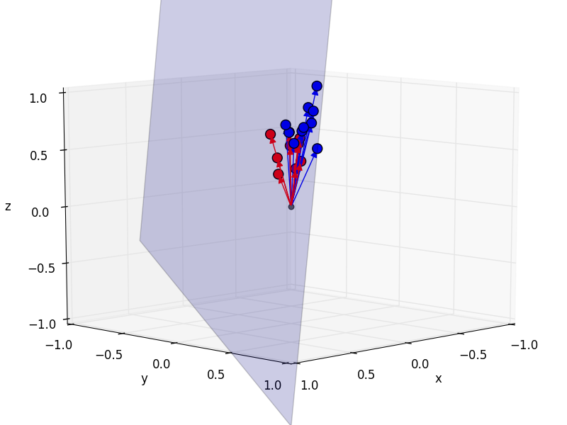
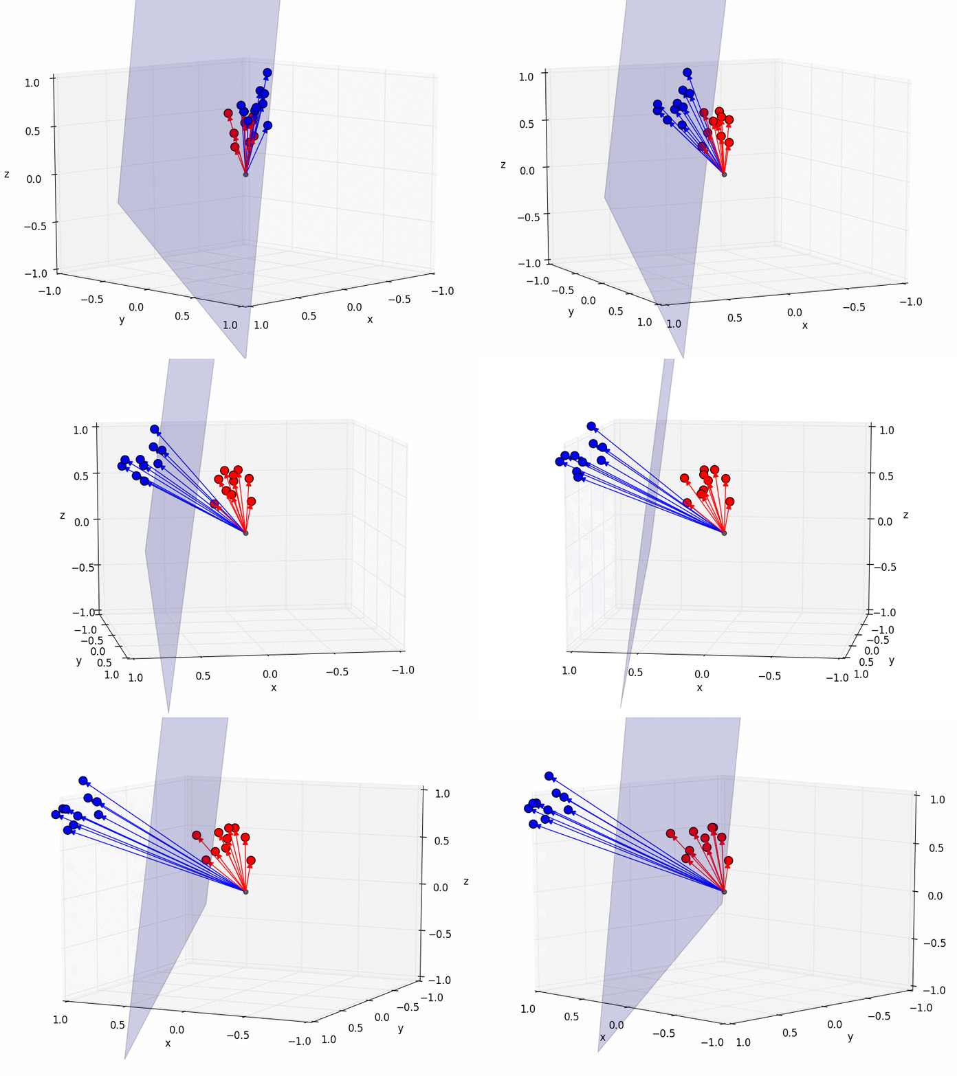
How could a computer automatically discriminate between these two categories? Geometrically, of course! By treating each image as a point in a 945-dimensional space, we can now come up with a geometrical interpretation of discriminating between categories: we find a plane which separates these two sets of points (blue is me, red the blobfish):

Using this plane, the computer can now automatically discriminate between blobfish and Sebastians by checking on which side of the plane the point lies.
Sit back for a second and make sure that you have understood this. Because if so you can be proud - you have just understood the key principle behind image classification, the problem that I have presented in the intro article! The majority of all approaches in machine intelligence draws such planes through the high-dimensional image space, assigns a category to each side of the plane, and then checks on which side of the plane a new, previously unseen image lies.
Caveats
Of course, there are some details that I have omitted. As mentioned before, the sketch is in 3 dimensions, although we should draw 945 dimensions, which is not possible; and also the thing separating the two object categories in 945 dimensions is not really a plane, but a hyperplane (that’s what a plane is called in four or more dimensions - not to be confounded with hyperspace). But still, the math - which I have not shown you, so you need to trust me on this one - assures us that the concepts of points and planes also exist in 945-dimensional space, so it is totally valid to think of it in 3 dimensions only.
Another important detail that I have omitted is how to find this (hyper-)plane. And in fact this is the central problem of machine intelligence, or more precisely machine learning. We will talk about how this learning works in the post after the next one.
Finally, I have to lower your expectations about this method a bit: discriminating Sebastians and blowfish by finding a plane in this 945-dimensional space does not really work well in practise. The reason is that pictures of Sebastians and blowfish are not as nicely separable as I have suggested in the 3D arrow picture above, but rather scattered all around the space. But the general idea of finding discriminating hyperplanes in high-dimensional spaces still holds. And we can get it to work by first bringing the image into a different representation, that is a different space, and then finding the hyperplane in this new space (at this point you should remember our discussion about representations in the previous post). You can either try to transform images in these representations explicitly, i.e. think of a good representation and program it yourself, or implicitly, trying to find a way of doing this automatically. We will talk about both approaches later, too.
Terminology
Some last notes on terminology.
Often, sequence of numbers, such as the 3d point or the 945-dimensional representation of the image is called a vector, and it then lives in a vector space of some dimensionality. Although being basically the same thing, the term vector has a slightly different connotation which we will ignore for now. But I will mostly use the vector mainly because it sounds cooler.
Secondly, mathematics tries to be parsimonious with concepts, mainly because it makes talking about things easier. Therefore, we get rid of the concept “numbers” by treating them as 1-dimensional vectors. So in the future if I talk about vectors, you can often think of them as just being numbers.
Summary
To summarize, the approach of machine intelligence is the following: we transform some input, for example an image into a table of numbers, call this a vector and then treat this vector as a point in a high-dimensional space. We then apply our knowledge of how to manipulate points in 3D to transform this high-dimensional vector in order to extract information from it. Moreover, we can classify between different types of data, for example object categories, by finding discriminating hyperplanes in this space.
In the next post we will look at how be more precise about what we mean by transformations and how to describe these hyperplanes by introducing the concept of functions.
TL;DR:
- Data can be viewed as points in high-dimensional spaces
- We can apply the same transformations to points in this space as in 3D
- Such points are called vectors
- Hyperplanes in space discriminate between vectors, and hence categories
Footnotes:
- Actually, linear algebra can do even a bit more than what is “physically possible” in the 3D world, e.g. mirroring and skewing objects.
- To turn images into an arrow/point, we need to remove the column and row structure of the image and write all of the numbers in one very long row. And since 27 times 35 = 945, the original image becomes a 945-dimensional point. This has indeed been common practise when learning from images (although more recent algorithms exploit the spatial, i.e. “grid” structure of the image, rather than just stitching the columns together).
- It is important to notice that moving or rotating a point in 945-dimensional space which represents an image is not the same as shifting or rotating the image! Since moving in 3D is equivalent to “adding a number to one or more dimensions”, this is also the definition of moving in 945-dimensional space. If you push a 3D object 3m up and 5m to the right you effectively add these two numbers some coordinates of the object. Hence, in the image example, moving is equivalent to changing the gray scale value of certain pixels. Neither do vector rotations actually rotate the image.

