Yet Another Machine Learning 101
This post is a somewhat short recap of machine learning in general. I wrote it as lecture notes for a tutorial that I gave in one of the robotics courses at TU Berlin.
It will probably be difficult to understand it in detail if you are a beginner. For beginners, I recommend reading my blog on intuitive machine intelligence.
The post is also available as an ipython notebook which allows you to play around with the python examples.
General setting
In general, we distinguish three general paradigms in ML
- Supervised Learning
- Unsupervised Learning
- Reinforcement Learning
Additionally, there is a variety of other paradigms, which are not going to be covered here, such as semi-supervised learning and learning from side information which will not be covered here.
In all types of machine learning the goal is to learn a function to predict some output from some input data:
\[f: X \rightarrow Y\]The different paradigms differ in
- the goal, i.e. what kind of data $X$ and $Y$ are
- the training data available to learn $f$
We will now review the different paradigms and give examples, however, mostly focusing on supervised learning.
Supervised Learning
Supervised learning is by far the most popular paradigm. In this setting, we are given examples from $X$ and $Y$, i.e. $N$ pairs ${ x^{(i)}, y^{(i)} }_{i=1\ldots N }$. The data $x^{(i)}$ are called the input data and $y^{(i)}$ the labels. Together, they are called the training data.
Any ML method usually consists of (at least) three ingredients.
- A representation of $f$, i.e. whether it is a linear function, polynomial, neural network, or non-parametric, etc.
- An appropriate loss function $\mathcal{L}$,
- which is minimized using an optimization method.
The loss function for supervised learning looks as follows:
\[f = \textrm{argmin}_{f}\ \mathcal{L} ( f, \{ x^{(i)}, y^{(i)} \}_{i=1\ldots N })\]A loss function can be thought of as an assessment of how good $f$ fits the training data. If its value is high, it means that $f(x^{(i)})$, i.e. our prediction of the label for $x^{(i)}$ given current function $f$, is very different from the known true value $y^{(i)}$. If $\mathcal{L} = 0$, it means the $f$ perfectly fits the data.
An optimization method can be thought of as a method that is given data and a loss function and automatically tries to find the best function minimizing the loss. There is a wide variety of optimization methods, and they mostly differ by the properties of $f$ they exploit (e.g. if $f$ is differentiable, we can compute its derivative, set it to zero, and go step by step in the direction of steepest descent; this is called gradient descent optimization, see below). We only look at some very basic optimization methods, but it is of course the success in learning a function greatly depends on the optimization used.
The representation of $f$ also drastically influences its learnability. The easiest and best-understood representations are linear functions, but also neural networks (which are some sort of nonlinear functions) are very common nowadays.
Usually, as a practitioner, you don’t have to worry about making choices these three things. An ML method usually determines the loss, optimization and function representation, and is tuned in such a way that all of them work together nicely.
Overfitting
We said that the goal of supervised learning is to learn a function $f$ from training data, using the loss $\mathcal{L}$. However, it is important that a perfect loss, $\mathcal{L}=0$, for your training does not necessarily solve the problem – the actual task of supervised learning is to learn an $f$ that generalizes to unseen examples $x^{(j)}$. And actually, fitting the training data is very easy: just memorize all of them by heart! This will trivially give us $\mathcal{L}=0$ for our training data. But as we will see, that might mean that for unseen data we will actually make blatantly wrong predictions.
To repeat, the core problem of any machine learning method is to learn an $f$ that generalizes to unseen data. If $f$ only works well on the training data, but not on unseen data, we say $f$ overfits the data.
To ensure that our function does not overfit, we divide the data into three sets:
- Training data
The data used for actually learning/fitting the function - Validation data
Additional data, not used for learning the function, but only used to compute the loss for our current estimate of the function. It is also used to tune the hyperparameters of your method, or decide which ML method to use. - Test data
Another additional data set, neither used for training nor for validation. You can think of it as being locked in some secret drawer, and it is only released and used to evaluate $f$ once you are sure that you have properly learned $f$.
Example: Linear regression
Let us consider a simple example for supervised learning: linear regression.
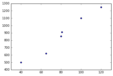
Assume we want to predict the price of apartments in Berlin, given their size of square meters of the apartment. Here is some fictitious data:
| $X$ (square meters) | $Y$ (monthly rent in Euro) |
|---|---|
| 40 | 500 |
| 65 | 620 |
| 80 | 855 |
| 81 | 910 |
| 100 | 1100 |
| 120 | 1250 |
Let’s plot the data
In [1]:
%pylab inline
set_printoptions(suppress=True)

X = array([40, 65, 80, 81, 100, 120]).reshape((-1, 1))
Y = array([500, 620, 855, 910, 1100, 1250])

scatter(X, Y);
Populating the interactive namespace from numpy and matplotlib
The idea is linear regression is to fit a linear function, i.e. a line of the form $f(x) = w_1 x + w_0$ to the data. To learn such a line we define as loss the mean-squared error which penalizes large deviations of $f(x)$ from the known $y$:
\[\mathcal{L}_\textrm{MSE} = \frac{1}{2N} \sum_{i=0}^N ( f(x^{(i)}) - y^{(i)})^2\\ = \frac{1}{2N} \sum_{i=0}^N ( w_1 x^{(i)} + w_0 - y^{(i)})^2\]Maybe you are a bit confused about the fraction $\frac{1}{2N}$. The reason we use it, because if we compute the derivative $\mathcal{L}_\textrm{MSE}$, the square within the sum cancels out this fraction; and the $\frac{1}{N}$ normalizes for the number of training examples.
Note that usually $x$ is multi-dimensional, i.e. a vector $\mathbf{x}$. Then $w_1$ becomes a weight vector $\mathbf{w}$. We can do another trick to get rid of $w_0$ (called the bias or intercept term) by appending a $1$ to $\mathbf{x}$, and extending $\mathbf{w}$ by one dimension. This facilitates notation a bit, as it allows us to write the loss using vector notation:
\[\mathcal{L}_\textrm{MSE} = \frac{1}{2N} \sum_{i=0}^N ( \mathbf{w}^T \mathbf{x}^{(i)} - y^{(i)})^2\]Gradient descent
How to optimize it? One way is to compute the partial derivative wrt. each $j$-th element of the weight (the so-called gradient), and change the updates:
\[\nabla \mathcal{L}_\textrm{MSE} = \frac{\partial \mathcal{L}_\textrm{MSE}}{\partial {w}_j} = \frac{1}{2N} \sum_{i=0}^N \frac{\partial}{\partial {w}_j} ( \mathbf{w}^T \mathbf{x}^{(i)} - y^{(i)})^2 \\ = \frac{1}{2N} \sum_{i=0}^N 2 w_j^{(i)} (w_j x_j^{(i)} - y^{(j)})\\ = \frac{1}{N} \sum_{i=0}^N w_j (f(x_j^{(i)}) - y^{(j)})\]The gradient descent algorithm (for linear regression with MSE) then goes as follows:
- Initialize the weights $\mathbf{w}$ randomly
- Update each $j$-th entry in the weight vector by following the negative
gradient:
$w_j^\textrm{new} = w_j - \alpha \frac{1}{N} \sum_{i=0}^N w_j (f(x_j^{(i)}) - y^{(j)})$
Here, $\alpha$ denotes the step size. It has to small enough, otherwise we might overshoot and miss the minimum.
If we image the loss function to be a “bowl” and every $\mathbf{w}$ to be a
point in this bowl, the gradient points towards the bottom of this bowl, and
thus the minimum of the loss. The update rule then takes small steps towards
this minimum.
This is a cool visualization which is also accompanied by a Matlab
script:

Gradient descent is a very important technique, very popular especially for training neural networks (see below).
Ordinary least squares
In the linear regression case, however, there is a more direct solution. If we consider $\mathbf{w}$ to be a matrix rather than a vector, we can write the loss in the following way:
\[\mathcal{L}_\textrm{MSE} = \frac{1}{2} (\mathbf{X}\mathbf{w} - \mathbf{y})^T (\mathbf{X}\mathbf{w} - \mathbf{y})\]where $\mathbf{X}$ contains in each $i$-th row on training example $\mathbf{x}^{(i)}$, and $\mathbf{y}$ in each $i$-th row a label $y^{(i)}$.
Now we can compute the derivative of $\mathcal{L}_\textrm{MSE}$, set it to 0, and solve for $\mathbf{w}$. As you can check yourself, the derivative is given by: \(\frac{d \mathcal{L}_\textrm{MSE}}{d \mathbf{w}} = \mathbf{X}\mathbf{w} - \mathbf{y} \\ \mathbf{X}\mathbf{w} - \mathbf{y} = 0\\ \mathbf{X}\mathbf{w} = \mathbf{y}\)
To now solve it for $\mathbf{w}$, we need to invert $\mathbf{X}$ – which is usually not possible because it is not square in the general case. But we can apply a trick, namely use the pseudo-inverse:
\[\mathbf{X}\mathbf{w} = \mathbf{y}\\ \mathbf{X}^T\mathbf{X}\mathbf{w} = \mathbf{X}^T\mathbf{y}\\ \mathbf{w} = (\mathbf{X}^T\mathbf{X})^{-1} \mathbf{X}^T\mathbf{y}\\\]where the pseudo-inverse is given by $(\mathbf{X}^T\mathbf{X})^{-1} \mathbf{X}^T$.
Computational example
Let’s now implement this in python.
In [2]:
# transpose training data and append 1
Xhat = np.hstack([X, np.ones((X.shape[0],1.))])
w = np.linalg.inv(Xhat.T.dot(Xhat)).dot(Xhat.T).dot(Y)
w
array([ 10.04581152, 58.78926702])
In [3]:
scatter(X, Y)
plot(X, Xhat.dot(w));
Luckily, there are libraries that do all that for us. One of the most popular ML libraries in python is scikit learn. We can easily verify that it computes the same function:
(we see that sklearn automatically adds a bias, stored in the variable “intercept_”)
In [4]:
from sklearn.linear_model import LinearRegression
lr = LinearRegression()
lr.fit(X, Y)

X_rng = np.linspace(40, 120, 100).reshape((-1,1))

scatter(X, Y)
plot(X_rng, lr.predict(X_rng));
lr.coef_, lr.intercept_
(array([ 10.04581152]), 58.789267015706741)
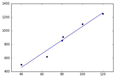
We see that the weights and our prediction (the blue line) are identical. And you see that it fits the data Ok, but not perfectly. Still, it looks like a reasonable guess. Most importantly, it also makes a prediction for inputs $x$ for which we did not have any training data.
Overfitting
What if we don’t want to fit a line, but some more complex model, e.g. a polynomial? This is easily done by augmenting our input (also called feature expansion) by different powers of the input:
$f(\tilde{\mathbf{x}}) = [\mathbf{x}, \mathbf{x}^2, \mathbf{x}^3, … ]$
Let’s try that out:
In [5]:
def polynomial_feature_expansion(X):
    return np.hstack([X, X**2, X**3, X**4, X**5,])

X_rng = np.linspace(20, 140, 100).reshape((-1,1))

lr = LinearRegression()
lr.fit(polynomial_feature_expansion(X), Y)

scatter(X, Y)
plot(X_rng, lr.predict(polynomial_feature_expansion(X_rng)));
ylim(200, 2000)
lr.coef_, lr.intercept_
(array([ 14413.72962393, -394.63014472, 5.20499616, -0.03319069,
0.00008213]), -201202.688457913)
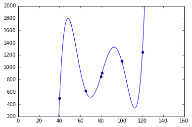
We see that the training data is fitted almost perfectly; but the function hallucinates weird values inbetween and before/after the training data! Also, the weights are actually very high. This is a classical example of overfitting: we used a function that is too “powerful”, as it has many more parameters than the linear model. There are different ways to remedy this problem:
- More training data!
- Restricting the function to a simpler one (e.g. less parameters)
(The danger can be underfitting, i.e. choosing a too simple model) - Model selection, e.g. using cross-validation
- Incorporating prior knowledge about the problem, e.g. by feature engineering
- Regularization
At this point we will only talk about regularization which a special way to force a powerful function not to overfit. The idea is to put additional terms into the loss function. A popular regularization is L2 which puts a L2-norm penalty on the weights, i.e. $||\mathbf{w}||^2$ into the loss. The optimizer then has to make sure not only to fulfill the initial loss, e.g. the mean-squared error, but also the regularization.
A linear regression with L2 regularization is called ridge regression. The loss then becomes: \(\mathcal{L}_\textrm{Ridge} = \frac{1}{2} (\mathbf{X}\mathbf{w} - \mathbf{y})^T (\mathbf{X}\mathbf{w} - \mathbf{y}) + \alpha ||\mathbf{w}||^2\)
where $\alpha$ weights the influence of the regularizer.
Ridge regression is also implemented in scikit learn:
In [6]:
from sklearn.linear_model import Ridge

lr = Ridge(alpha=20.)
lr.fit(polynomial_feature_expansion(X), Y)

scatter(X, Y)
plot(X_rng, lr.predict(polynomial_feature_expansion(X_rng)));
ylim(200, 2000)
lr.coef_, lr.intercept_
(array([-0.05208327, -2.0080791 , 0.05283245, -0.00047523, 0.00000145]),
1401.9265643035942)
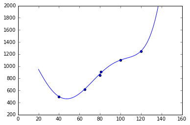
We see, that the weights are lower and the values inbetween are much smoother; but still for values $>120$ and $<40$ the linear model reflects our intuition about the real $f$ better. Therefore, we might choose to increase the regularization, collect more data or choose a different function parametrization, e.g. a polynomial with lower degree.
Regression vs. Classification
Before we talk about more sophisticated supervised learning methods, we should clarify the terms regression and classification. The only difference between these two concepts is whether $y$ is discrete or continuous. In the previous example we used regression, i.e. we treated the price as a continuous variable. In classification, we are usually given a discrete, finite set of classes, and we are only interested in predicting the class of a new input. The only thing that changes because of this is the loss. We won’t bother about these loss functions now, but in case you are interested, common choices are the categorical cross-entropy loss or the hinge loss.
But watch out, the terminology is not always fully consistent: training a linear model with a categorical cross-entropy loss is called logistic regression – although it is actually a classification method!
(Deep) Neural Networks
Currently, they are probably the most popular approach in supervised learning. The idea is to compose the function $f$ of small slightly nonlinear functions (neurons) and connect them. This small nonlinear functions are called neurons, and together they form a neural network that can be visualized as follows:

The picture (image taken from wikipedia) depicts a network with an input layer ($=\mathbf{x}$), an output (should be equal to our labels $y$) and a hidden layer. This hidden layer can learn some representation of $\mathbf{x}$ that is suitable for predicting $y$. For the record, this network structure is also sometimes called multi-layer perceptron.
What does a (non-input and non-output) neuron look like? In fact, a neuron basically multiplies a linear weight vector with its input (sounds exactly like linear regression, right?) and then applies some nonlinearity on the output of this operation (that’s different from linear regression). Let’s make this formal; a neuron $h_i$ (in the hidden layer), given input $\mathbf{z}$ (in the network above $\mathbf{z} = \mathbf{x}$), computes its output as follows:
\[h_i(\mathbf{z}) = \sigma(\mathbf{w}_{h_i}^T\mathbf{z})\]where $\sigma$ denotes some nonlinear activation function, often something like the sigmoid-function:
\(\sigma(t) = \frac{1}{1 + e^{-t}}\),

although the hyperbolic tangent and rectifiers are more en vogue in state-of-the art neural networks.
A hidden layer $f_h$ composed of $H$ neurons then computes its output as follows:
\[f_h(\mathbf{z}) = \sigma(\mathbf{W}_{h} \mathbf{z}),\]where ${\mathbf{W} _ h}$ is a $\mathrm{dim}(\mathbf{z}) \times k$ matrix composed of the stacked (transposed) weight vectors $\mathbf{w}_{h_i}^T, i=1 \ldots H$, and the activation function $\sigma$ is applied separately to each output dimension of $\mathbf{W}_H$.
So what are deep networks? The idea is to stack multiple hidden layers – the more hidden layers there are, the “deeper” the network is. Mathematically, it is just a repeated application of multiplying a linear weight with the output of the previous layer, then computing the activation, passing it to the next layer, and so on. The advantage of these networks is, that they can learn more sophisticated representations of the input data, and thus solve more challenging learning problems.
Finally, we have to say how to train neural networks. We can use the same loss functions as for linear regression (or classification, of course), and apply gradient descent. However, if we have multiple layers, we need to apply some tricks to adapt gradient descent. The first trick is backpropagation; it basically says that to train multiple layers, we apply gradient descent to each layer separately, and pass the loss backwards through the network layer by layer until we reach the beginning. For this to work well, we must apply also some additional tricks, e.g. setting the initial values of all weights appropriately and so on. But in principle, training a neural network is not much different from performing a linear or logistic regression.
Of course there is a lot more to know abouot deep learning, and if you want a more in-depth treatment of this topic, check out this recent book.
Unsupervised Learning
Unsupervised differs from supervised learning that we are only given ${x^{(i)}}_{i=1 \ldots N}$, an no labels. This obviously means that the loss functions we’ve seen so far will not work. Instead the loss functions impose some “statistical” constraints on $y$. A good example is Principal component analysis (PCA): here we want to learn a low-dimensional variant of $x$ – however, which still contains roughly the same “information” as the original $x$. The question is how to quantify “information”. This very complicated and highly depends on the task; but PCA takes a pragmatic stance by defining information as high variance (in a statistical sense). Therefore, the loss for PCA is roughly equivalent to:
\[{\mathcal{L}}_\textrm{PCA} \approx -\textrm{Var}(f(\mathbf{x}))\]where $f$ is indeed a linear function as used above. The $\approx$ sign reflects that formally the loss is a bit different - we need some additional constraints to make this problem well-defined, i.e. not find infinitely large weights. I will not go into details here, but you should understand that one can formulate learning objectives without any supervised signal, just by formulating some desired properties of the result of $f$ in the loss function.
Note that PCA is somewhat the “regression” variant of unsupervised learning. There are also methods that map data into discrete representations, e.g. in clustering. The most popular and yet simplest method is probably k-means.
Also note that unsupervised learning has somewhat different applications than supervised learning. Often it is used for pre-processing the input data, in order to then feed its output to a supervised learning method. Another important application is exploratory data analysis, i.e. studying and finding patterns in your data.
Reinforcement Learning
In reinforcement learning our outputs $Y$ are actions that an agent should take, and our input X is the state. Therefore, we also rename $X$ and $Y$: the state is denoted by $\mathbf{s}$, the actions by $\mathbf{a}$, and the function we want to learn is called policy $\pi$ (instead of $f$):
\[\pi(\mathbf{s}) = \mathbf{a}\]A crucial difference to supervised learning is that we do not know the correct actions $\mathbf{a}$. Rather, we only get a reward signal $r(\mathbf{s}, \mathbf{a})$ for every action we take (in a certain state). The reward is a real number that is high if the action was good, and low if it was bad.
Obviously, this problem is much harder as learning becomes indirect – you need to figure out the right action only from getting a reward. The biggest problem is that rewards are usually sparse and delayed; that means the agent might receive a positive reward only after it has executed a set of actions. However, it might be that actually the first action in this sequence was the most important one.
There is a wide variety of different techniques, such as policy search, value-based methods and model-based reinforcement learning to tackle this problem. We will look at these techniques at this point, but it is important that you at least understand the general setting of reinforcement learning, and its difference to supervised learning (and unsupervised learning).